Potential of Mean Force (PMF) version updated for Amber 24
This is a minor modification from the previous tutorial, as from Amber24 the Adaptive String Method is included in by default. So no manual modifications to the code are needed anymore.
The main file-related changes are these two:
Firstly, you no longer need STRING file.
Secondly, some changes to the input files are required. Specifically, you must include an ‘&asm’ section and the ‘asm = 1’ keyword in the ‘&ctrl’ section. You will see these changes throughout the tutorial.
Adaptive Finite Temperature String Method in Collective Variables.
In this tutorial, we will explore an efficient and practical approach to acquiring the free energy profile along a reaction coordinate for complex chemical reactions, eliminating the requirement for multidimensional free energy surfaces. By simply providing a guessed path for the chemical reaction, the string method will effectively identify the closest minimal free energy path within the specified degrees of freedom in chemical space. Also, you don’t need to have identified the exact position of the reactants and product structures for this method, as the string method is able to find them.
Before we begin, I highly recommend checking out the tutorial written by Kirill Zinovjev in his GitHub repository. This tutorial is specifically designed to replicate the reaction mechanism proposed in the original paper of this methodology. The system under consideration is small enough to be tested within a time frame of less than half an hour on a single cluster node. Furthermore, in that tutorial, you will gain insights into how the method operates when employing a combination of bonds and angles as collective variables (CVs). As for our particular case, we will solely be utilizing distances as our CVs.
0. Introduction
Roughly speaking, a reaction mechanism provides a logical and detailed description of the steps involved in transforming a given set of reactants into another set known as products. This transformation is associated with an energy landscape, and the reaction predominantly takes place along the minimal free energy path (MFEP) that connects the regions of reactants and products. These regions are separated by their corresponding transition state.
Exploring the free energy landscape and accurately describing a chemical reaction becomes more challenging as the number of involved coordinates increases. Initially, when only a single coordinate, such as forming or breaking a bond, is considered, the task is relatively simple from a computational standpoint. However, during the course of a chemical reaction, multiple coordinates can serve as Collective Variables (CVs) to describe the process. These can include bond lengths, bond orders, bond angles, dihedrals, or changes in atom hybridizations.
The complexity arises when a larger number of coordinates are needed to fully explore the free energy landscape and provide an accurate description of the chemical reaction. In such cases, bidimensional or even three-dimensional free energy surfaces become necessary. In real systems, the number of required coordinates can reach unmanageable levels, resulting in significant computational demands. This challenge stems from constructing a multidimensional free energy surface to represent the reaction, with computational costs growing exponentially alongside the number of involved coordinates. This phenomenon is commonly referred to as the curse of dimensionality.
The problem becomes more tractable when we shift our focus from the entire free energy surface to the region of interest known as the minimal free energy path (MFEP). With the string method, we can incorporate any number of Collective Variables (CVs) to obtain the MFEP without sacrificing efficiency. However, the bottleneck in this approach is similar to other methodologies like QM/MM, which involves considerations of the QM region’s size and the chosen level of theory to describe it.
According to the Transition State Theory, the activation free energy (\({\Delta{G^{\ddagger}}}\)) (that is, the highest energy along the path) is related to the experimental catalytic constant (\(k_{cat}\)) by the following expression:
\(k_{cat}=\frac{K_BT}{h}e^{(-\frac{\Delta{G^{\ddagger}}}{RT})}\)Where:
\({k_{cat}}\) has s-1 units,
\({K_B}\) is the Boltzmann constant (\({1.38\times10^{-23}J\cdot K^{-1}}\)),
\({T}\) is the temperature in Kelvin,
\({h}\) is the Planck constant (\({6.63\times10^{-34}J\cdot s}\)),
\(\Delta{G^{\ddagger}}\) is the activation free energy (\({J\cdot mol^{-1}}\)), and
\(R\) is the gas constant (\({8.314\,J\cdot mol^{-1}K^{-1}}\)).
If the \({\Delta{G^{\ddagger}}}\) along this path agrees with the measurements in the lab (\(k_{cat}\)), the reaction mechanism proposed is likely describing what is happening at the atomic level.
Try yours in the following \({\Delta{G^{\ddagger}}}\) / \(k_{cat}\) calculator:
1. Method
The reaction primarily occurs along a specific path in the multidimensional space of reaction coordinates, known as the “reaction tube.” This forms the foundation of the path-based approach method, which effectively addresses the challenge of describing the reaction mechanism using multiple variables.
Assuming that this process takes place within a narrow region encompassing most of the reactive trajectories connecting reactants and products, the progress of the reaction can be represented by a single path Collective Variable (CV) without losing essential information. This path-CV describes the system’s advancement along the minimal free energy path (MFEP) and serves as the reaction coordinate (RC) for studying the process.
It’s important to note that a string calculation involves two stages. The first stage entails the evolution of the string to locate the MFEP. The second stage involves defining the path-CV, often denoted as ‘s’. Once this path is established, an Umbrella Sampling calculation is conducted along this coordinate to obtain the Free Energy Profile of the reaction (also known as the Potential of Mean Force or PMF). To move from the first to the second stage requires stopping the evolution of the string once it has found the MFEP, and this will be explained in further detail later.
I encourage you to read the publication on this methodology to gain a broader perspective of its implementation https://pubs.acs.org/doi/10.1021/acs.jpca.7b10842
2. Chemical reaction
Since this tutorial is aimed at intermediate-advanced Amber users, I will skip the system preparation process and the protocol for running classical molecular dynamics simulations. However, if you are not familiar with these basics, you can first learn them from Amber introductory tutorial.
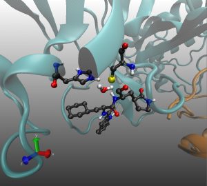
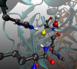
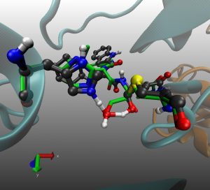
In this tutorial you will find the way to obtain the minimal free energy pathway for the mechanism of inhibition of the SARS-CoV-2 main protease by the inhibitor PF-00835231 (see doi.org/10.1002/anie.202110027).This reaction is a perfect example to show how the string method can deal with a complex collective variable. Here the reaction coordinate is obtained as a combination of 7 CVs (see Fig. 1).
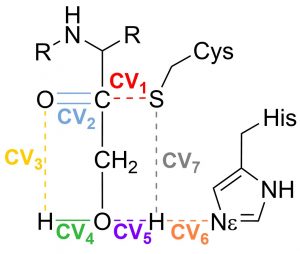
Fig. 1 Set of Collective variables used to describe the reaction coordinate
This proposal begins by exploring the formation of the Cys/His ion-pair intermediate, with the proton transfer process described by CV7 and CV6. Once the ion-pair structure is established, the cysteine-sulfur undergoes a nucleophilic attack on the inhibitor’s carbonyl carbon (CV1). This sulfur attack is concerted with the double proton transfer: from the His to the hydroxyl group (CV6 and CV5), and from the hydroxyl group (CV4) to the oxygen in the carbonyl group (CV3).
Next, we provide a brief overview of each file used to run the string method in Amber (please note that this tutorial assumes the use of a customized Amber installation, as described in Section 1). As you progress through this tutorial, each of these files will be explained in detail.
3. Files
-
-
-
- CVs : contains the information about the atoms involved in every collective variable that form the set of CVs.
- guess : contains the initial path that roughly describes the reaction mechanism.
- in : this is a template to be used as input for every string node.
- in.sh : is a bash scripts to create the Amber’s string.groupfile and the input file for every node.
- string.groupfile: the group file needed to run multiple independent simulations in Amber.
- string.sh: this is an example to submit the simulations in a machine using the slurm workload manager.
- STOP_STRING: this file is manually created once the string has found the MFEP. It contains the time interval (in simulation steps) during which the force constants and reaction coordinate “s” are averaged. These averaged values are then used to generate the final_parameters.dat file, which contains the necessary information for obtaining the PMF. (This file will be described in detail in the section 4)
-
-
To begin with, we require at least two structures—one for the reactants and one for the products—described with the same Hamiltonian. It is crucial that these structures are pre-equilibrated at the QM/MM level of theory before usage. While it is a general recommendation in molecular dynamic simulations, having a well-equilibrated system provides better control over the overall process. Ideally, a structure for each intermediate is also necessary. This facilitates the generation of structures for the string nodes during the preparation step.
All files are Amber files:
Then, we define the set of CVs that describe the reaction progress. Here we have a CV set with 7 distances.
3.1. CVs
To understand this file, note that the first line specifies the number of collective variables describing the chemical reaction. Each collective variable is represented by a separate $COLVAR block. The COLVAR_type keyword indicates the type of variable, such as “BOND,” “ANGLE,” “DIHEDRAL,” or “PPLANE.” The atoms keyword includes the Amber indices of the atoms associated with the specific COLVAR_type. For distances, two indexes are used; for angles, three indexes; and for dihedrals and planes, four indexes are utilized. Additionally, comments after the indexes will help to identify the variable being described (optional). Finally, in some $COLVAR blocks, there may be an optional box keyword that constrains the collective variable within a specified range, typically to prevent the string from getting lost in diffusion processes.
7
$COLVAR
COLVAR_type = "BOND"
atoms = 2242, 4674      !S····C=O
box = 1.3, 4.0
$END

$COLVAR
COLVAR_type = "BOND"
atoms = 4674, 4675      !C=O
$END

$COLVAR
COLVAR_type = "BOND"
atoms = 4675,   4678    !C=O····HO
$END

$COLVAR
COLVAR_type = "BOND"
atoms = 4678,  4677     !H-O inh
$END

$COLVAR
COLVAR_type = "BOND"
atoms = 4677,   618     !HO····HEHis
$END

$COLVAR
COLVAR_type = "BOND"
atoms = 618, 617        !His.HE-NE.His
$END

$COLVAR
COLVAR_type = "BOND"
atoms = 2242, 618       !S····HEHiS
box = 1.0, 4.0
$END
Next we have to define roughly the reaction mechanism pathway.
3.2. guess
In this file we will propose our hypothesis for the reaction mechanism pathway:
5
        3.20    1.20    3.00    1.00    3.20    2.00    1.30
        2.80    1.25    2.85    1.00    2.60    1.50    1.30
        2.40    1.30    2.70    1.00    2.05    1.00    2.20
        2.00    1.35    1.40    1.21    1.40    1.00    3.00
        2.00    1.40    1.00    2.53    1.00    1.80    3.00
The first line indicates the number of steps used to describe the reaction, which is five in this case. Following that, each subsequent line represents the values of the collective variables (CVs) at each step. Each column corresponds to a specific CV, and each row represents a different step.
Typically, the values for the CVs in the reactants, products, or any stable intermediate steps are obtained by averaging their values from previous molecular dynamics simulations at those specific steps. While it is recommended, this approach is not mandatory. If these values are obtained in this manner, the ends of the string can be fixed, meaning their values remain constant throughout the simulation. This can be specified in the STRING file.
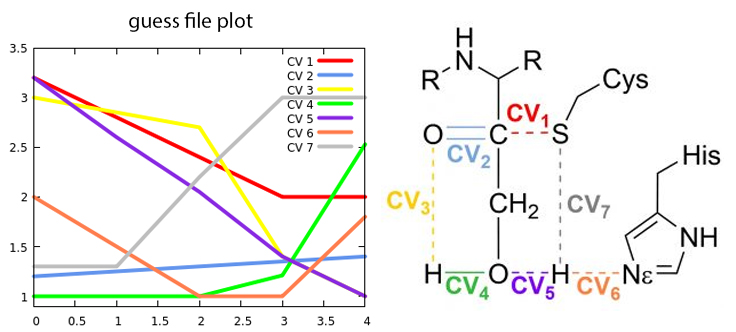
Fig. 2 Change in the collective variables from reactants to products
The first step in the reaction mechanism according to the initial guess shown in Figure 2 is the proton transfer from Cysteine to Histidine (CV7····CV6). The H-S bond (grey line) only starts to be broken when the H is close enough to be transferred to the \(N_\epsilon\) in the histidine (orange line).. We call this intermediate the Ion Pair (IP).
After the IP is fully formed, the proton in the hydroxymethyl group of the inhibitor begins to approach the oxygen in the carbonyl group (represented by the green and yellow lines corresponding to CV4 and CV3, respectively). Simultaneously, the recently transferred proton undergoes another transfer, this time from histidine to the oxygen atom (depicted by the orange and purple lines denoting CV6 and CV5). The nucleophilic attack of the cysteine sulfur on the carbonyl carbon occurs in coordination with these proton transfers (represented by the red line corresponding to CV1).
3.3. in
This is a standard input file for Amber. It does not contain any information specific to the string method. The string method is activated only when the STRING file is present in the working folder. The “ig = XXXXX” value will be replaced with a random value during the calculation, ensuring that the calculation can be replicated if needed.
QM/MM Gaussian interface MD

&cntrl
  imin      = 0,        ! Minimization off
  ntf       = 1,        ! Bond interactions involving H-atoms evaluated, SHAKE is not performed, use with NTC=1
  temp0     = 300.0,    ! Reference temperature at which the system is to be kept
  tempi     = 300.0,    ! Initial temperature
  ntt       = 3,        ! Switch for temperature scaling. Use Langevin dynamics with the collision frequency γ given by gamma_ln
  irest     = 0,        ! no restart a simualtion
  ntx       = 1,        ! Reading only coordinates from the restraint file
  ntb       = 1,        ! Volume constant
  cut       = 8.0,      ! Non bonded cut
  gamma_ln  = 5.0,      ! Collision frequency
  nstlim    = 1000000,  ! Steps, for 1 ns
  dt        = 0.001,    ! Every step of 1 fs
  ntpr      = 50,       ! Print the progress every ntpr steps
  ntwx      = 50,       ! Every ntwx steps, the coordinates will be written to the mdcrd file.
  ntwr      = 50,       ! Every ntwr steps during dynamics, the restrt file will be written
  ntxo      = 1,        ! Format of the final coordinates,
  ifqnt     = 1,        ! Switch on QM/MM coupled potential
  asm       = 1,        ! Adaptive String Method
  ig        = XXXXX
/
  &qmmm
  qmmask ='@609-620, 2239-2242, 4654-4658, 4674-4681', !index 608 to 619 2238 to 2241 4653 to 4657 4673 to 4680
  qmcharge=0,
  qm_theory='DFTB3',
  writepdb  = 1, !QM region will be written on the very first step to the file qmmm_region.pdb
  qmcut=8
/
&asm
  guess_file = 'guess',
/
In the &asm section additional keywords can be include, for example:
- dir is the directory is where the files containing the string information will be saved.
- z_bias can be set either to .true. or .false. It controls the orthogonal bias during the potential of mean force (PMF) phase (default .true.)
- preparation_steps determines the number of steps used to increase the force constant value for each collective variable (CV) from the starting structure to the configuration given in the guess file (1ps, so 1000 steps if time step is 1 fs).
- CV_file is the path to the file to the CVs file, (default CVs).
- REX_period specifies the frequency at which replica exchange will be attempted during the string or PMF phase (default 50 steps if time step is 1fs).
Additionally, there are other optional keywords that can be included to modify the frequency at which the string writes certain outputs:
- output_period specifies that information or files will be printed in the results folders every output_period steps (default is 100,).
- buffer_size is the interval range used to compute the PMFs along the string and the frequency of integration along the PMF phase (default 2000)
If the string have already converged and you want to submit only the PMF phase, you must include the following keyword in the STRING file:
- only_PMF = .true. it performs the PMF stage only and not the string evolution, (default is .false.)
For more information, please refer to page 492 of the Amber24 manual.
3.4. in.sh
This script generates the group file necessary for the calculation. It is in this file that the structures of the reactants and products will be specified.
In the calculation, the first half of the string nodes will use the structure of the reactants as their starting point, while the second half of the nodes will use the structure of the products. In this particular example, 48 string nodes will be utilized, with each node running on a separate CPU.
execute it by typing:
sh in.sh 48
in.sh file content:
#!/bin/bash

# If groupfile exists, remove it
if [ -f string.groupfile ];
then
  rm string.groupfile
fi

PARM=parameters.parm7  # path to topology file
REACT=reactants.rst7   # path to reactants structure
PROD=products.rst7     # path to products structure

# Number of string nodes is provided as command line argument
nodes=$1
for i in $(seq 1 $nodes); do
  # generate sander input for node $i
  sed "s/XXXXX/$RANDOM/g" in > $i.in

  # use reactants structure for the first half of the nodes and products for the rest
  if [ $i -le $((nodes/2)) ];
  then
    crd=$REACT
  else
    crd=$PROD
  fi

  # write out the sander arguments for node $i to the groupfile
  echo "-O -rem 0 -i $i.in -o $i.out -c $crd -r $i.rst7 -x $i.nc -inf $i.mdinfo -p $PARM" >> string.groupfile
done
echo "N REPLICAS  = $i"
After executing this script with the number of nodes specified as a parameter (in this case, 48), it will create 48 input files, one for each simulation. Additionally, it will generate the string.groupfile .
3.5. string.groupfile
Each line in this file will submit a simulation for each node.
-O -rem 0 -i 1.in -o 1.out -c reactants.rst7 -r 1.rst7 -x 1.nc -inf 1.mdinfo -p parameters.parm7
-O -rem 0 -i 2.in -o 2.out -c reactants.rst7 -r 2.rst7 -x 2.nc -inf 2.mdinfo -p parameters.parm7
.
.
.
-O -rem 0 -i 47.in -o 47.out -c products.rst7 -r 47.rst7 -x 47.nc -inf 47.mdinfo -p parameters.parm7
-O -rem 0 -i 48.in -o 48.out -c products.rst7 -r 48.rst7 -x 48.nc -inf 48.mdinfo -p parameters.parm7
3.6 string.sh
The content of this file will depend on the architecture of your cluster machine (for example, in a SLURM environment, here it was named “string.sh“). Regardless of the specific details, the file should include the following essential information:
#!/bin/bash
export I_MPI_COMPATIBILITY=3

mkdir results

mpiexec sander.MPI -ng 48 -groupfile string.groupfile
At this point if everything goes well your string simulation must be running and if it had already finished the preparation step phase we can start analysis how it is searching for the MFEP of our chemical reaction.
4. STRING ANALYSIS
First things first. Check that the string is running, inside the 1.out you should find something like this
---String method------------------
Number of CVs                    7
Number of nodes                 48
Node                             1
----------------------------------
Also, in the results folder the files 1.dat to 48.dat should have been created.
As long as nothing is written in the .dat files the calculation will be running the preparation steps. That means the force constants for every CV in every node are increasing to reach the optimal value before starting the search for the minimal free energy path. In this way the next analysis can be made only once the phase of the preparation steps has been finished, 2000 step in this example. Nevertheless in order to gain a real insight about how the string is evolving it would be better to wait at least until the first preliminary .PMF be written, 2000.PMF in this case.
Inside the results folder are stored all the files to be used to check the evolution of the string or the PMF obtained during the PMF phase.
At any moment of the simulation you can check the integrity of the structures by checking if the “vlimit exceeded” message appears in some .out file using the next command:
for i in {1..48};do echo ${i}; grep 'vlimit exceeded' ${i}.out | tail -n 1;done
If there is something wrong with a structure, check the .rst7 corresponding to the number printed above the vlimit exceeded message. If nothing is printed means that the structures are OK.
If everything is OK, the string is looking for the MFEP. We can move now to the results folder to check the evolution of the string.
4.1 Convergence
To check if the string is still moving and observe its convergence you can plot the ‘convergence.dat’ file stored in the results folder using a tool like gnuplot using the following command:
plot 'convergence.dat' w l
This plot will provide visual insights into whether the string has found the minimal free energy path (MFEP). It is expected to display a pattern similar to the following example:
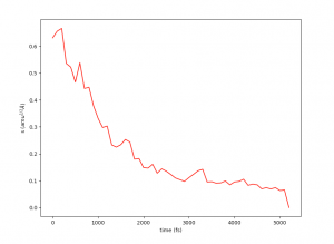
The convergence of the string to its minimal free energy path (MFEP) can be determined by observing the reaction coordinate over time. If there are no significant changes in the reaction coordinate, and it remains fluctuating near a specific value (e.g., 0.1), it indicates that the string has converged. In this specific case, this behavior has been observed for 3000 steps (equivalent to 3 picoseconds).
Once the string has converged, you can proceed to the potential of mean force (PMF) phase by creating the “STOP_STRING” file within the results folder. For instance, in this case, the “STOP_STRING” file will contain only two lines, with the numbers 3000 and 5000, representing the region where the convergence remains close to 0.1. If everything is in order, the required final files for running the PMF phase will be generated after the subsequent simulation state, including files such as “0_final.string,” “final_parameters.dat,” “1_final.dat,” and so on.
4.2 Visualization of the changes in the CVs during the convergence of the string
While the string is progressing towards its minimal free energy path (MFEP), we can observe the evolution of the collective variables (CVs) throughout the process. Every 100 steps, a “step_number.string” file will be generated. These files have similar characteristics to the guess file, where each column represents a CV, and each line corresponds to the value of that CV for each node of the string.
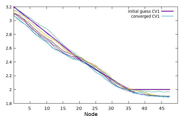
Here is an example illustrating the evolution of CV1. The initial guess for CV1 is depicted in bold purple. The 0.string file contains interpolated values for each string node, providing more accurate representations. The values of CV1 gradually change as the string converges from the initial guess to the final 5000.string file, which is illustrated by the bold blue/cyan line.
plot '0.string' u 1 w l lw 2 title 'initial guess CV1'
replot for [i=200:4800:200] ''.i.'.string' u 1 w l notitle
replot '5000.string' u 1 w l lw 2 title 'converged CV1'
Now the same can be made for every CV, or if you prefer you can plot all at once with the next gnuplot command.
plot for [i=3000:5000:500] for [j=1:7] ''.i.'.string' u j w l notitle
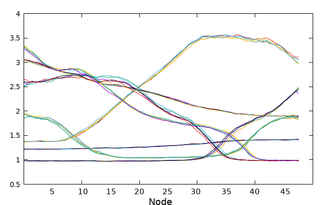
To avoid cluttering the plot, only the values of the collective variables (CVs) taken every 500 steps in the converged region are plotted. This selective plotting helps to maintain clarity and prevents overcrowding of the graph when all data points are plotted simultaneously.
4.3 Replica exchange and structure sorting
To ensure that the structures are sorted back to their initial positions as replica exchange is being performed, follow these steps:
- Create a folder to store the sorted structures.
- Inside that folder, execute the following Python script:
#!/usr/bin/env python3

import os

if os.path.exists('../results/plot_final.REX'):
    plot = 'plot_final.REX'
else:
    plot = 'plot.REX'

with open(f'../results/{plot}', 'r') as f:
    idx = f.readlines()[-1].split()[1:]

for i in range(len(idx)):
    print(f'{i+1} is now {idx[i]}')
    os.system('cp ../' + str(i+1) + '.rst7 ' + idx[i] + '.rst7')
With the structures sorted, you can use VMD to examine how the reaction is occurring loading the visual.vmd file by typing in the bash console:
vmd -e visual.vmd
Please take into account that the visual file needs to be placed in the same folder as the parameters.parm7 file. Within this folder, make sure to include a ‘sorted’ folder containing the restart files.
additionally if you have problems using the VMD visualisation file you can follow these steps:
- Load the “parameters.parm7” file in VMD.
- Open the VMD TkConsole.
- Type the following command in the TkConsole to add the structures corresponding to every string node:
for {set i 1} {$i < 49} {incr i} {
mol addfile path/to/sorted/structures/${i}.rst7 type rst7 waitfor -1
}
Replace “path/to/sorted/structures” with the path to the folder where you stored the sorted structures. This command will loop through each string node and add the corresponding structure to the VMD display.
Once you with your structures loaded, you will be able to visualize the structures corresponding to each string node in VMD, allowing you to observe the reaction’s progression.
This an example of what you will observe, your visualization will look less smooth, as it is a minimisation along the reaction coordinate. It was created solely for visualisation purposes.
To assess the performance of replica exchange, you can plot the data from the plot.REX file (or plot_final.REX during the PMF phase) using gnuplot or similar tools. Here’s an example command to plot the file:
plot for [i=2:49] 'plot.REX' u 1:i w l lw 2 notitle
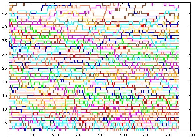
Please note that white spots in the plot indicate areas where the sampling could be improved. If the structures are OK, these white spots will disappear as the simulation progresses and more sampling is performed.
Moving forward, you can examine the preliminary potential of mean force (PMF) files that have been written. These files contain valuable information about the energy landscape and the reaction pathway. By analyzing the PMF files, you can gain insights into the thermodynamics and kinetics of the chemical reaction.
4.4 Plotting the .PMF files.
During the evolution of the string, within the “results” folder, a “buffer_size.PMF” file will be generated every buffer_size steps. These files provide a rough approximation of the potential of mean force (PMF) and will continue to change as the simulation progresses. It is important to note that these files should be used cautiously and only to obtain a preliminary understanding of the thermodynamics and kinetics of the chemical reaction. For more accurate and reliable results, it is recommended to wait for the final PMF files generated at the end of the simulation.
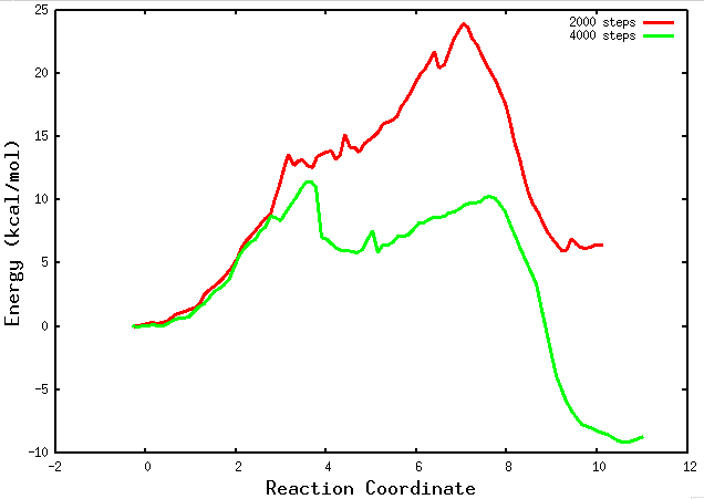
Inside the results folder you can plot those preliminary files using gnuplot:
plot for [i=2000:4000:2000] ''.i.'.PMF' u 1:6 w l lw 3 title ''.i.' steps'
If your string has converged and you are in the final PMF stage, a path collective variable (path-CV) is defined using the MFEP that was found. At this point, you will begin to observe the “buffer_size_FINAL.PMF” files. These files contain information about the PMF obtained along the reaction coordinate. They provide valuable insights into the energy landscape and the thermodynamics of the chemical reaction. Analyzing these files will allow you to examine the energetics and barriers along the reaction pathway.
You can plot the “buffer_size_FINAL.PMF” files in the same way as you plotted the preliminary PMF files during the string phase.
It is crucial
to note that this tutorial has provided a basic understanding of the string method and its implementation. Further exploration, experimentation, and refinement are encouraged to adapt the approach to specific systems and research goals. The string method offers a powerful tool to unravel the reaction mechanisms, thermodynamics, and kinetics of complex chemical reactions, paving the way for advancements in various fields, including computational chemistry, drug discovery, and materials science.
Possible problems and solutions
P1: There are no minima in reactants and products region in the PMF
S1: Check if there is a CV trying to go to a further distance than the one in the ‘box’ defined in the CVs file. If so, increase the box range and resubmit the string using now as initial guess the values in the last XXXX.string files written. Also, you can use as initial structures the last structures obtained from the previous calculation. Remember, they have to be sorted previously in case you used replica exchange.
S2: Check that there are not a restraints interfering the evolution of CVs freely.
S3: Force the Collective Variables (CVs) to take higher or lower values than they should in the reactant and product regions, and fix the ends of the string.
P2: The PMF are not smooth and present jumps, they are ‘spiky’
S1: Integrate the final.dat files using Alan Grossfield WHAM. you will need to transform the string final.dat files into something WHAM can understand using the convert_dat.py file. You need to transform one by one. I recommend to create a WHAM folder inside the results folder and run a a bash for loop for this
for i in {1..48}; do ./convert_dat.py ../${i}_final.dat > $i.dat; doneWhere 48 is the total number of node you are using.
S2: check the sampling for each collective variable. there is a column for each CV in every final.dat. the sampling fro CV1 is in column 3 for CV2 in column 4 and so on. The following jupyter notebook will help you with this task. put the notebook in the same folder were the final.dat files are.
Recent Comments